Exploring Villager Music Taste in Animal Crossing New Horizons
The world is a grim place right now. But there has been one beacon of shinning light in the darkness. That’s right - Animal Crossing: New Horizons. The game has developed into a phenomenon with it’s chill and charming atmosphere providing light relief and escapism in the form of hefty loan repayments to an anthropomorphic racoon.
Part of the game’s charm stems from it’s soundtrack and given my own growing suite of work analysing music in video games - it made sense to dig a little deeper into the music of the Animal Crossing world.
K.K. Mania
For those who haven’t played the game, Animal Crossing New Horizon’s is a life simulator, placing you on a desert island which you can harvest resources from to develop into a blooming island paradise along with your other villagers - a set of NPCs with whom you share the island. The NPCs each have their own charachters and one aspect of that charachter is their music preference. In the Animal Crossing world, there’s one musician that everybody loves - K.K. Slider. K.K is a genre spanning dog. He’s the George Harrison of the Animal Crossing world and his diverse back catalogue contributes to hs wide appeal. So that begs the question: What villager attributes influence their favourite K.K. Slider track?
The Data
Thankfully, there was a recent dataset uploaded to Kaggle that includes villager attributes from the game so we’re going to use that to conduct the analysis. There’s a wide range of other csv files with different types of game data in there too so go check it out if you’re interested.
head(villagers)## # A tibble: 6 x 17
## Name Species Gender Personality Hobby Birthday Catchphrase
## <chr> <chr> <chr> <chr> <chr> <chr> <chr>
## 1 Admi… Bird Male Cranky Natu… 27-Jan aye aye
## 2 Agen… Squirr… Female Peppy Fitn… 2-Jul sidekick
## 3 Agnes Pig Female Big Sister Play 21-Apr snuffle
## 4 Al Gorilla Male Lazy Fitn… 18-Oct ayyyeee
## 5 Alfo… Alliga… Male Lazy Play 9-Jun it'sa me
## 6 Alice Koala Female Normal Educ… 19-Aug guvnor
## # … with 10 more variables: `Favorite Song` <chr>, `Style 1` <chr>, `Style
## # 2` <chr>, `Color 1` <chr>, `Color 2` <chr>, Wallpaper <chr>,
## # Flooring <chr>, `Furniture List` <chr>, Filename <chr>, `Unique Entry
## # ID` <chr>The main reason we chose this dataset is that it already has a ‘Favourite Song’ column that we can use as an outcome variable to try and predict. Let’s check it out in more detail.
villagers %>%
  ggplot(aes(x=reorder(`Favorite Song`,`Favorite Song`,
                       function(x)-length(x)))) +
  geom_bar(aes(fill = stat(count))) +
  coord_flip() +
  theme_minimal() +
  scale_fill_continuous() +
  theme(axis.title.y = element_text(size = 12, colour = "#000000"),
        axis.title.x = element_text(size = 12, colour = "#000000"),
        axis.text.y = element_text(size = 5, colour = "#000000"),
        axis.text.x = element_text(size = 5, colour = "#000000"),
        plot.background = element_rect(colour = "#FAFAFA", fill = "#FAFAFA"),
        panel.background = element_rect(colour = "#FAFAFA", fill = "#FAFAFA"),
        strip.background = element_blank(),
        legend.position = "none"
  )+
  labs(y = "Favourite Frequency",
       x = "Song",
       caption = "Data from the Kaggle 'NookPlaza' dataset - LonelyManOfData")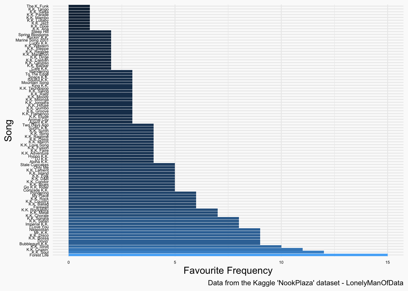
Okay - firstly, I knew the developers had gone to great lengths to write a tonne of K.K. Slide songs but I didn’t realise there’s be this many. There’s only just under 400 villagers (or rows in our dataset), I doubt we’re going to be able to do any fancy predictive modelling here based on the sheer span of songs (although fair play to the devs for writing so many songs for a musical dog).
One thing we can do is start exploring some of the other characteristics in the data to see if any seem to suggest a relationship with favourite song.
Exploring Villager Attributes
Personality
villagers %>%
  ggplot(aes(x=reorder(`Favorite Song`,`Favorite Song`,
                       function(x)-length(x)))) +
  geom_bar(aes(fill = Personality)) +
  coord_flip() +
  theme_minimal() +
  scale_fill_viridis_d() +
  theme(axis.title.y = element_text(size = 12, colour = "#000000"),
        axis.title.x = element_text(size = 12, colour = "#000000"),
        axis.text.y = element_text(size = 5, colour = "#000000"),
        axis.text.x = element_text(size = 5, colour = "#000000"),
        plot.background = element_rect(colour = "#FAFAFA", fill = "#FAFAFA"),
        panel.background = element_rect(colour = "#FAFAFA", fill = "#FAFAFA"),
        strip.background = element_blank()
  )+
  labs(y = "Favourite Frequency",
       x = "Song",
       caption = "Data from the Kaggle 'NookPlaza' dataset - LonelyManOfData")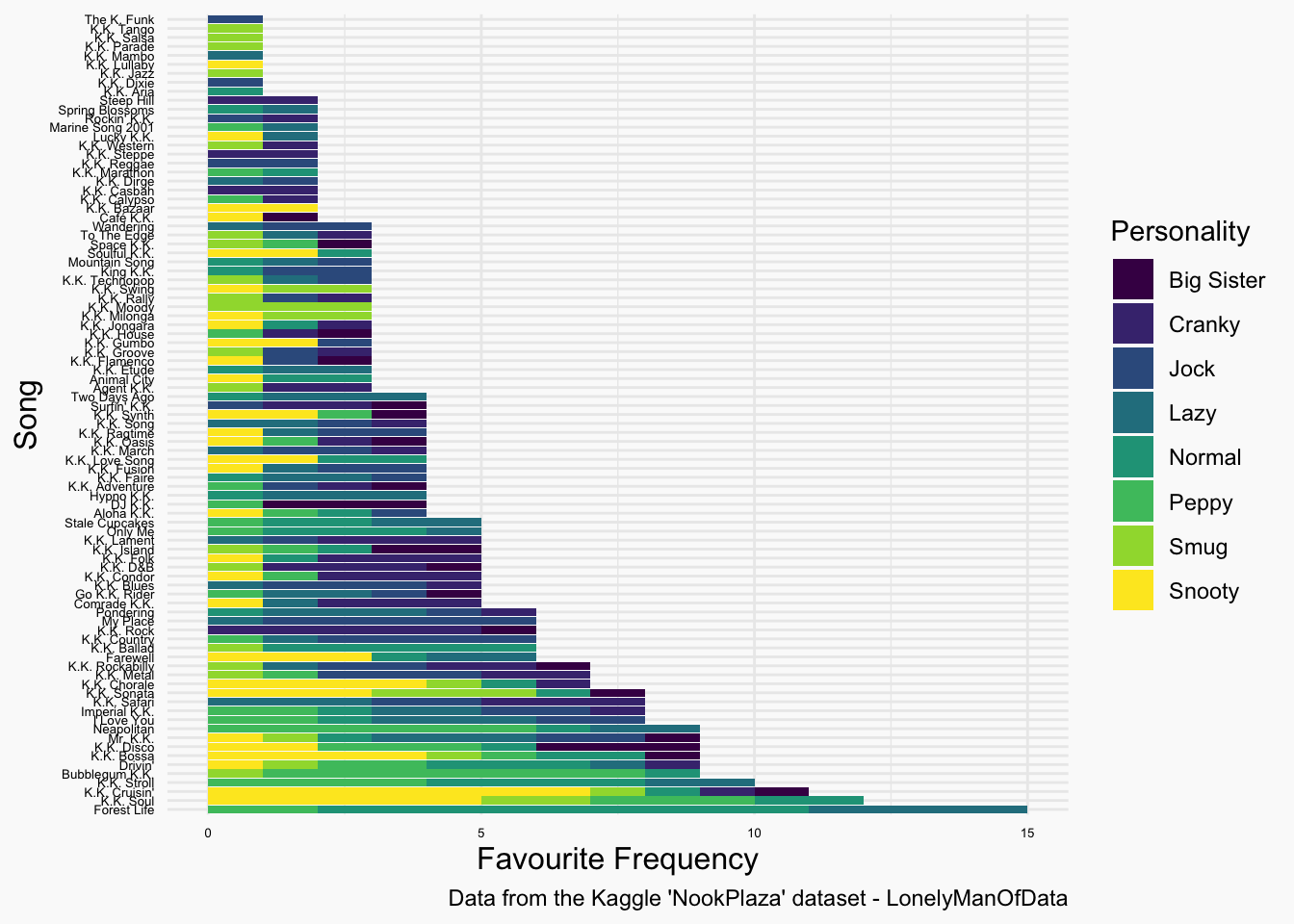
Personality often dictates what genres of music people like in reality - perhaps it’s the same for the Animal Crossing villagers. Forest Life, the most popular track, seems to appeal to those of a Normal personality. Perhaps this is a reflection of how mainstream music appeals to the avergae member of the populus? Or maybe I’m completely over analysing this…Then again, K.K. Rock is liked by those of a cranky disposition. I think there’s enough here to suggest the devs had some kind of thought process to tie personality with music taste when developing the characters.
Hobby
villagers %>%
  ggplot(aes(x=reorder(`Favorite Song`,`Favorite Song`,
                       function(x)-length(x)))) +
  geom_bar(aes(fill = Hobby)) +
  coord_flip() +
  theme_minimal() +
  scale_fill_viridis_d() +
  theme(axis.title.y = element_text(size = 12, colour = "#000000"),
        axis.title.x = element_text(size = 12, colour = "#000000"),
        axis.text.y = element_text(size = 5, colour = "#000000"),
        axis.text.x = element_text(size = 5, colour = "#000000"),
        plot.background = element_rect(colour = "#FAFAFA", fill = "#FAFAFA"),
        panel.background = element_rect(colour = "#FAFAFA", fill = "#FAFAFA"),
        strip.background = element_blank()
  )+
  labs(y = "Favourite Frequency",
       x = "Song",
       caption = "Data from the Kaggle 'NookPlaza' dataset - LonelyManOfData")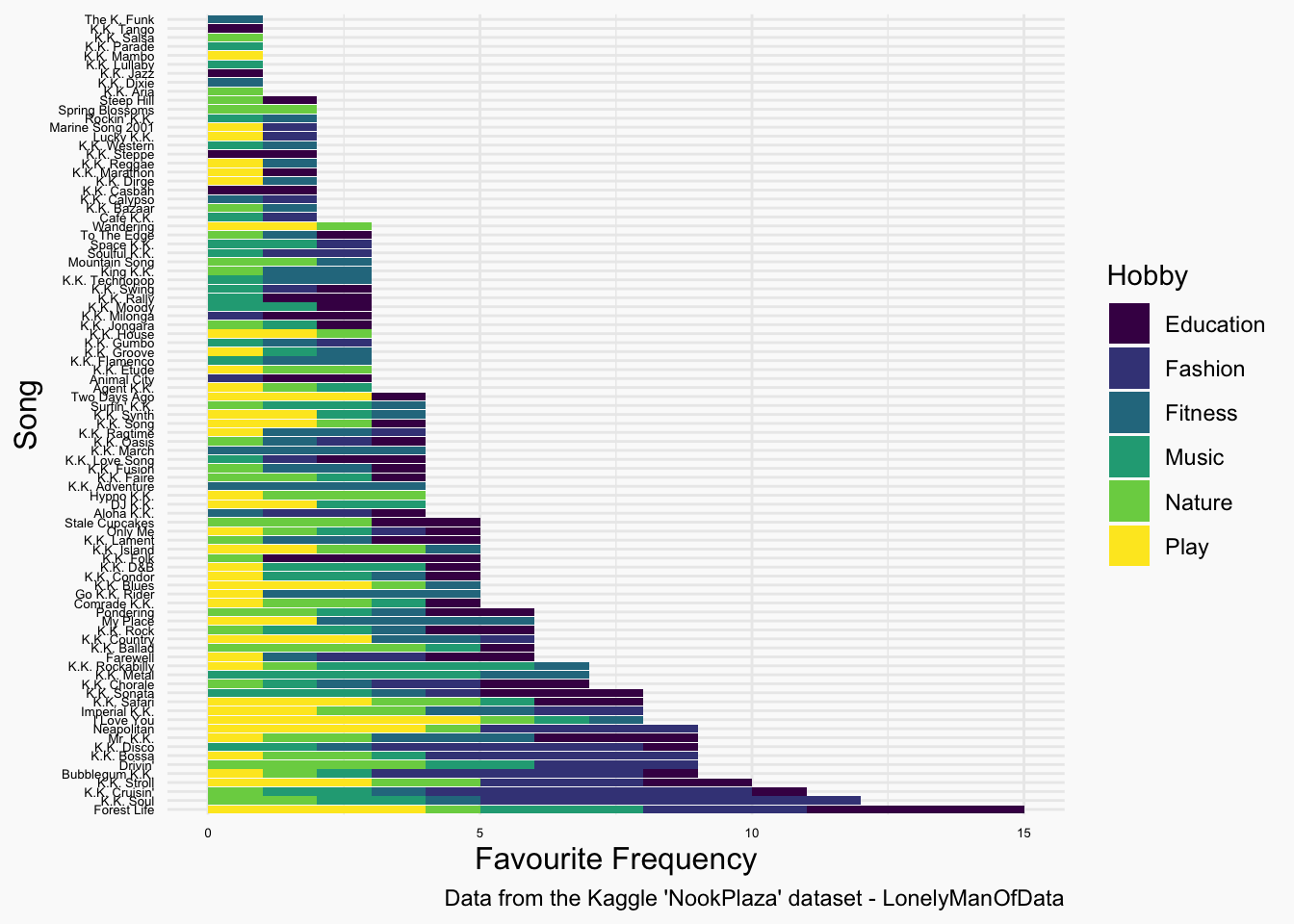
Villager hobby seems to have some legs as a predictor too. The Fashion hobby seems to tie in with the more ‘trendy’ and popular tracks, and the Music hobby is more niche genres like Metal and Rockabilly. There’s definetely some sort of pattern for the Play hobby too - although I’m not sure what it is on the surface. Perhaps there’s something about those tracks that is more inherently ‘fun’ or upbeat.
villagers %>%
  ggplot(aes(x=reorder(`Favorite Song`,`Favorite Song`,
                       function(x)-length(x)))) +
  geom_bar(aes(fill = Gender)) +
  coord_flip() +
  theme_minimal() +
    scale_fill_manual(
    values = c(
      Male = "#4477AA",
      Female = "#CC6677"
    )
  )+
  theme(axis.title.y = element_text(size = 12, colour = "#000000"),
        axis.title.x = element_text(size = 12, colour = "#000000"),
        axis.text.y = element_text(size = 5, colour = "#000000"),
        axis.text.x = element_text(size = 5, colour = "#000000"),
        plot.background = element_rect(colour = "#FAFAFA", fill = "#FAFAFA"),
        panel.background = element_rect(colour = "#FAFAFA", fill = "#FAFAFA"),
        strip.background = element_blank()
  )+
  labs(y = "Favourite Frequency",
       x = "Song",
       caption = "Data from the Kaggle 'NookPlaza' dataset - LonelyManOfData")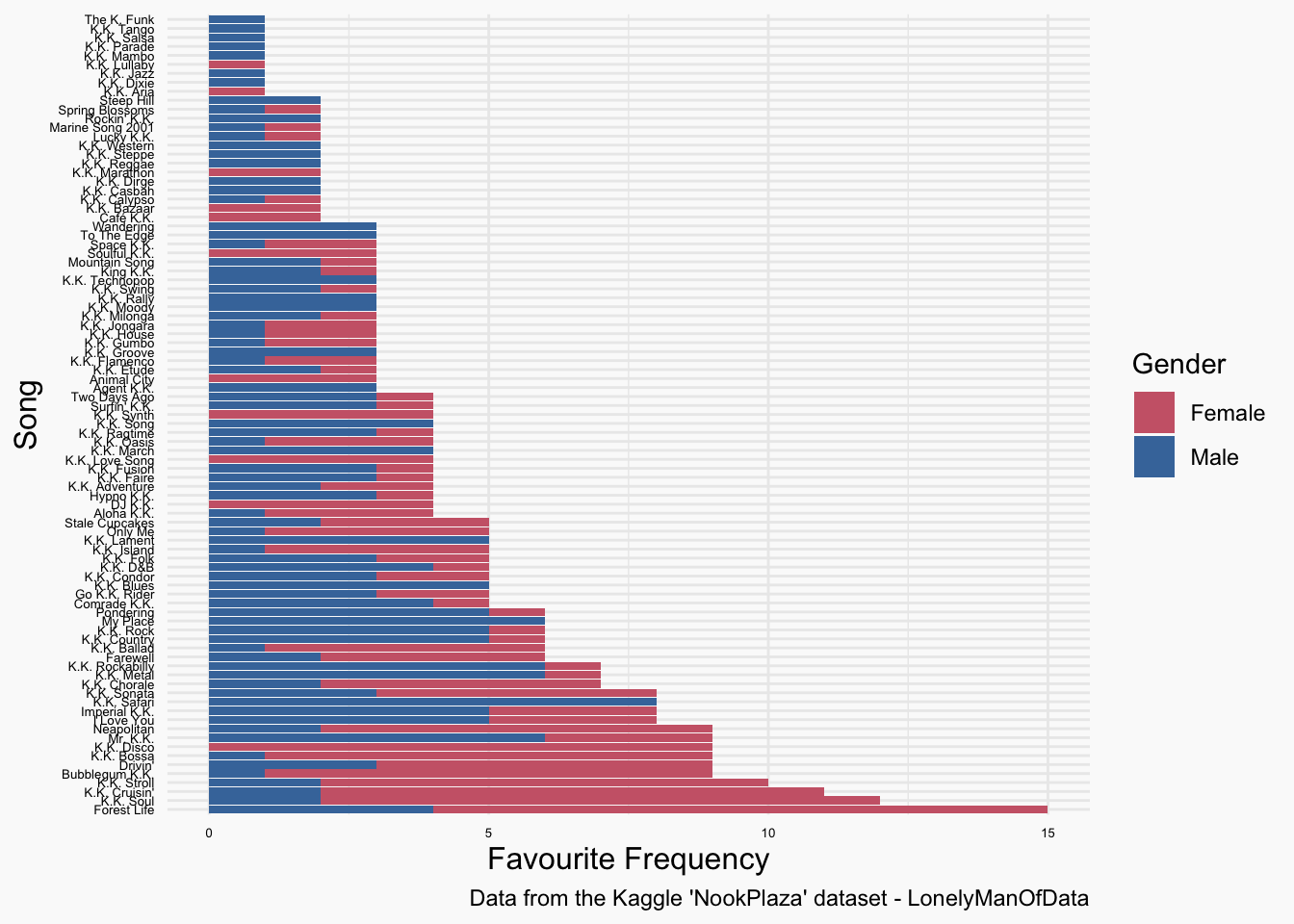
Once again, there are some tracks that are clearly differentiated by a male v female split. Female charachters appear to prefer K.K. Disco where as the dudes tend to like tracks like K.K.Sonata. But finding any pattern between these differences is tricky.
Species
villagers %>%
ggplot(aes(Species, `Favorite Song`)) +
stat_bin2d(aes(fill=..count..)) +
theme_minimal() +
scale_fill_viridis_c("Count",
breaks = c(1,2,3)) +
theme(axis.title.y = element_text(size = 12, colour = "#000000"),
axis.title.x = element_text(size = 12, colour = "#000000"),
axis.text.y = element_text(size = 5, colour = "#000000"),
axis.text.x = element_text(size = 7, angle = 45, colour = "#000000"),
plot.background = element_rect(colour = "#FAFAFA", fill = "#FAFAFA"),
panel.background = element_rect(colour = "#FAFAFA", fill = "#FAFAFA"),
strip.background = element_blank()
)+
labs(y = "Song",
x = "Species",
caption = "Data from the Kaggle 'NookPlaza' dataset - LonelyManOfData"
)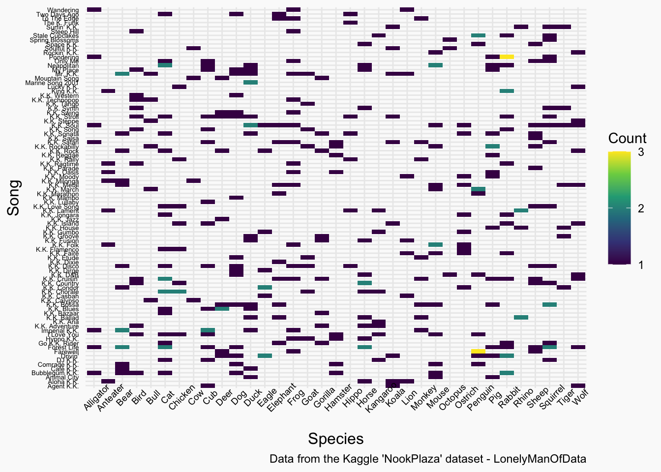 Species highlights the issue the data fairly well. There are so many songs and so many species, that there a load of gap counts. You have some songs that are only liked by one or two charachters so therefore, are only liked by one or two species. That said, within each species, music choice does seem to vary a fair bit. My guess is that if we built a model with the variables we’ve examined, we’d see Species be highly predictive and the rest be slightly predictive for this reason. Let’s see…
Making a Model
Note - If we we’re to build a more formal model - we’d probably do more feature engineering like grouping songs togther based on Genre or centrain types of Species together like mammals, amphibians etc. But since we’re only having a bit of fun, let’s build a model using the Random Forest method.
Random Forest works well here as we’re dealing with discrete variables and classification by way of a decision tree methods suits our purpose well - we’re trying to categorise favourite song by way of our other discrete variables. If we build the model and visualise the feature importance, this is what we get…
importance    <- importance(model_rf)
varImportance <- data.frame(Variables = row.names(importance),
                            Importance = round(importance[ ,'MeanDecreaseGini'],2))

# Create a rank variable based on importance
rankImportance <- varImportance %>%
  mutate(Rank = paste0('#',dense_rank(desc(Importance))))

# Use ggplot2 to visualize the relative importance of variables
ggplot(rankImportance, aes(x = reorder(Variables, Importance),
                           y = Importance, fill = Importance)) +
  geom_bar(stat='identity') +
  geom_text(aes(x = Variables, y = 0.5, label = Rank),
            hjust=0, vjust=0.55, size = 4, colour = 'red') +
  labs(x = 'Variables') +
  coord_flip() +
  theme_minimal() +
  labs(caption = "Data from the Kaggle 'NookPlaza' dataset - LonelyManOfData") +
  theme(plot.background = element_rect(colour = "#FAFAFA", fill = "#FAFAFA"),
        panel.background = element_rect(colour = "#FAFAFA", fill = "#FAFAFA"))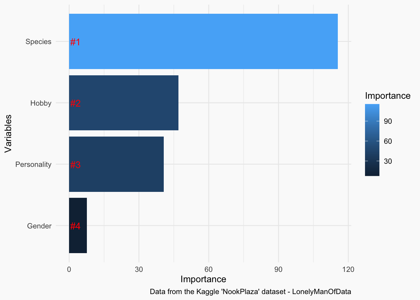
I wasn’t far off in my hunch. Species proves to be the mose important feature when determining music taste in Animal Crossing. I’m surprised at Gender being so comparatively low, but it just goes to show, K.K. Slider’s appeal transcends gender boundaries.
If we we’re being formal with the analysis, we’d dive into the model’s decision making criteria a bit deeper but at this point, I think we’ve a) more than over analysed Animal Crossing and b) we’ve answered the core research question. We’ve got enough evidence to clearly show that the developers clearly put thought into what determines villager music taste. Given the amount of little charming details in the game, I can’t say I’m surprised.
Summary
Dark times call for light entertainment. Animal Crossing New Horizons certainly provides a bucket load of that and analysing villager music tastes has provided me some. I was supposed to be at E3 around about now. Hopefully the event will run and I can make it next year. In the meantime, I’m going to continue delving into video game music analysis with R. Any suggestion for future articles, please do let me know.